---

Results July 26

S4D

A continuous-time first-order linear system per channel, diagonalized so that \(A\) is diagonal and the recurrence is elementwise:

\(\dot h(t) = A h(t) + B x(t), \qquad y(t) = \mathrm{Re}\,(C h(t)) + D x(t), \qquad A = \mathrm{diag}(a_1,\dots,a_N) \in \mathbb{C}^{N \times N}\)

Discretized by Zero-Order Hold with a fixed, learned step \(\Delta\):

\[\bar A = \exp(\Delta A), \qquad \bar B = A^{-1}\big(\exp(\Delta A) - I\big) B\]

Each \(a_n = \nu_n + i\omega_n\) is damped oscillator: Magnitude \(\mathrm{Re}(a_n) < 0\) sets memory length, \(\mathrm{Im}(a_n)\) sets frequency. \(\Delta, B, C\) are static => the layer is LTI=>=> the whole sequence is one convolution, computable by FFT.

Initialization:

• S4D-Lin: \(\nu_n = \tfrac12,\ \omega_n = \pi n\) => imaginary, filterbank.
• S4D-Real: \(\nu_n = n,\ \omega_n = 0\) => real, no oscillation, just decay due to exponential.

LinOSS

LinOSS switches to a second-order ODE:

\[h''(t) = -A\,h(t) + B x(t), \qquad y(t) = \mathrm{Re}\,(C h(t)) + D x(t), \qquad A = \mathrm{diag}(a_1,\dots,a_N) \succeq 0\]

Substituting \(z = h'\) gives a first-order system in \([z, h]\) of size \(2N\). The continuous-time poles are

\[\nu_{n} = 0,\qquad \omega_n = \sqrt{A_n}, \qquad a_n = \pm i\,\omega_n\]

The second-order system requires ODE integrators instead of Zero-Order Hold. With static \(\Delta\) and \(\gamma_n := \Delta\sqrt{A_n} = \Delta\,\omega_n\):

\[\lambda_n^{\mathrm{IMEX}} = \tfrac12(2 - \gamma_n^2) \pm \tfrac{i}{2}\sqrt{\gamma_n^2(4-\gamma_n^2)}, \qquad \lambda_n^{\mathrm{IM}} = \frac{1 \pm i\,\gamma_n}{1 + \gamma_n^2}\]

\[\lvert\lambda_n^{\mathrm{IMEX}}\rvert = 1, \qquad \lvert\lambda_n^{\mathrm{IM}}\rvert = \frac{1}{\sqrt{1+\gamma_n^2}} = \cos\big(\arg\lambda_n^{\mathrm{IM}}\big)\]

• Stability needs only \(A_n \ge 0\).
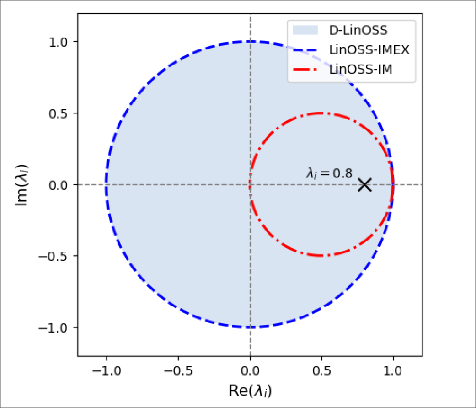
• IMEX is symplectic: \(\lvert\lambda_n\rvert = 1\) exactly, system never forgets.
• IM forgets, but its modulus is a fixed function of its phase: fast modes must decay fast, slow modes must decay slowly.
• Diagonal \(2\times2\) blocks => still a parallel scan, but no FFT convolution is used.

Problem: Damping is coupled to frequency, and comes from the integrator rather than the model. IMEX can't forget, IM can only forget at the rate its phase dictates. Neither can freely represent a pole. For example, \(\lambda = 0.8\) (real decay) lies on neither curve.

Solution: Dampened oscillator in continuous time system, with a second diagonal parameter \(G \succeq 0\):

\[h''(t) = -A\,h(t) - G\,h'(t) + B x(t)\]

\[\nu_{n}=\tfrac{G_n}{2},\quad \omega_{n}=\sqrt{A_n - \tfrac{G_n^2}{4}},\quad a_n = -\nu_n + i\,\omega_n\]

• \(A_n\) sets frequency, \(G_n\) sets decay.
• LinOSS is the \(G = 0\) case.

Discretizing with IMEX, and writing \(S_n = 1 + \Delta_n G_n\):

\[\lambda_n = \frac{1 + \tfrac{\Delta_n G_n}{2} - \tfrac{\Delta_n^2 A_n}{2}}{S_n} \pm \frac{\tfrac{\Delta_n}{2}\sqrt{(G_n - \Delta_n A_n)^2 - 4A_n}}{S_n}, \qquad \lvert\lambda_n\rvert = \frac{1}{\sqrt{1 + \Delta_n G_n}}\]

• The modulus depends on \(G_n\) only, phase on \(A_n\) only.
  • Damping and frequency are decoupled, and the reachable set is full unit disk.
• Stability is enforced via constraint:
  • \(\Delta = \sigma(\bar\Delta) \in (0,1)\)
  • \(G = \mathrm{ReLU}(\bar G)\)
  • \((G_n - \Delta_n A_n)^2 \le 4A_n\) .

Initialization

\((A_n, G_n) \mapsto \lambda_n\) is a bijection onto the punctured unit disk, so an eigenvalue distribution can be specified and solved back for the parameters:

\[A_n = \frac{\lvert\lambda_n\rvert^2 - 2\,\mathrm{Re}\,\lambda_n + 1}{\Delta_n^2 \lvert\lambda_n\rvert^2}, \qquad G_n = \frac{1 - \lvert\lambda_n\rvert^2}{\Delta_n \lvert\lambda_n\rvert^2}\]

Best-performing scheme: radially uniform \(\lvert\lambda_n\rvert \in [0.9, 1.0]\), uniform phase, then invert. This is the [[LRU]] annulus init reached by a different route.

Non-normal Transition

The LinOSS transition is modeled as a first-order recurrence via a non-normal block-diagonal matrix. This introduces possibility for transient growth of the state, even when eigenvalues are smaller than 1. Stability is guaranteed in the LTI case, but making components like \(G\), \(A\), \(\Delta_{n}\) time-varying makes the system unstable, even if eigenvalues are on the unit-disk.

Selective S4D-Real: Mamba

Mamba also uses Zero-Order Hold to discretize system, but step is input-selective.

\[\nu_n = \exp(\nu_n^{\log}), \qquad a_n = -\nu_n, \qquad \Delta_t = \mathrm{softplus}\big(s_\Delta(x_t) + b_\Delta\big)\]

\[\bar A_{t,n} = \exp(\Delta_t a_n) = \exp(-\Delta_t \nu_n), \qquad \bar B_{t,n} \approx \Delta_t B_{t,n}\]

• Since \(a_{n}\) is strictly negative, \(\Delta_{t}\) strictly positive => \(\bar A_{t,n} \in (0,1)\)
  • System is stable decay.
  • \(\Delta_{t}\rightarrow 0\) holds state, large \(\Delta_{t}\) resets state.
• \(\bar B_{t,n} \approx \Delta_t B_{t,n}\) is implementation only, not mentioned in paper.
• Since \(\Delta_{t}\) depends on \(x_{t}\), system is not LTI, requires associative scan.

Initialization: \(\nu_n^{\log} = \log n\) (so \(\nu_{n}\) is same as in S4D-Real)

Selective S4D-Lin: Oscillatory Mamba

Making LinOSS selective is difficult due to the non-normality of the transition, which makes it possible for transient growth to occur. However, Mamba formulation also works for complex-valued \(a_{n}\).

\[\nu_n = \exp(\nu_n^{\log}), \qquad a_n = -\nu_n + i\,\omega_n, \qquad \Delta_t = \mathrm{softplus}\big(s_\Delta(x_t) + b_\Delta\big)\]

\[\bar A_{t,n} = \exp(\Delta_t a_n) = \underbrace{\exp\!\big(-\Delta_t \nu_n\big)}_{\text{modulus}} \cdot \underbrace{\exp\!\big(i\,\Delta_t \omega_n\big)}_{\text{phase}}\]

• Modulus is unchanged to Mamba, eigenvalues are the same.
  • System is also stable.
  • Same time-step gating.
• Phase \(\omega_{n}\) needs no constraint, doesn't effect eigenvalue magnitude.
• Complex input force \(B\in\mathbb{C}^{1, N}\) and readout \(C\in \mathbb{C}^{N,1}\).

Selective Tuning

Problem: Phase is coupled to mode, can't tune mode selectively to input. For example, the model can't tune to changing pitch while keeping magnitude. Introducing a second \(\Delta_{\theta}\) term so that \(\exp(-\Delta_t \nu_n) \cdot \exp(i\,\Delta_{\theta} \omega_n)\) looses continuous-time formulation => SSM can't adapt to differing STFT framerates.

Solution: Add input-dependent phase-offset so that model can selectively adapt to input.

\[a_{t,n} = -\nu_n + i\,\big(\omega_n + \Delta\theta_t\big)\]

\[\bar A_{t,n} = \exp(\Delta_t a_{t,n}) = \underbrace{\exp\!\big(-\Delta_t \nu_n\big)}_{\text{modulus}} \cdot \underbrace{\exp\!\big(i\,\Delta_t (\omega_n + \Delta\theta_t)\big)}_{\text{phase}}\]

The offset is also multiplied by time-step, so changing the framerate scales everything consistently. Still stable since only phase-angle is touched, modulus stays unchanged.

Initialization

For \(\nu_{n}\) same initialization as in Mamba.

For \(\omega_{n}\) we choose \(\theta_{\max}\), then distribute \(\omega_{n}\) linearly from \(0\) to \(\theta_{\max}\) around unit disk. To get more Mamba-like behavior, we can choose \(M\) real-modes (setting \(\omega_{n<M}=0\)) and distribute the rest around the unit disk.

Since - \(B\) projects into complex domain - Real modes apply no phase change, only scale real and imaginary part. - \(C\) reads complex state. => Real modes act as independent real SSMs with shared decay. => Model learns to introduce rotation

Setting half the modes to real (\(M=N//2\)) gives best results.