Theory
The theory chain behind the selective-oscillatory-SSM proposal, in order: control-theoretic background, the stability proof for selective LinOSS, a survey of concrete SSM parameterizations, and the resulting S-LinOSS proposal.
Stability Background
Background control-theory for the LinOSS stability analysis below.
Lyapunov Stability
Motivation
For a Linear Time-Invariant (LTI) system, stability is often proven by analyzing the eigenvalues \(\lambda\) of the system matrix. For instance, in continuous-time systems, we require the real parts of all eigenvalues to be strictly negative (\(\text{Re}(\lambda_k) < 0\) for all \(k=1,\ldots,m\)).
However, in the case of a non-normal system matrix (where the eigenvectors are not orthogonal), standard eigenvalue analysis can mask problematic behaviors. Even if all eigenvalues satisfy the stability condition, the lack of orthogonality can lead to transient growth, meaning the state's magnitude may initially spike before eventually decaying. If the system is non-linear, this temporary spike might push the state outside the safe linear operating region. Therefore, a more robust stability proof is required: one that ensures the system trajectories from all possible initial states remain bounded and asymptotically approach an equilibrium state.
Definition
Lyapunov stability addresses this by guaranteeing that for any chosen maximum radius \(\epsilon > 0\), there exists an initial radius \(\delta > 0\) such that if the system starts within \(\delta\) of the equilibrium, it will never exceed the distance \(\epsilon\) over time:
This guarantees that for any small perturbation from the equilibrium state, the system's reaction is strictly bounded.
- Uniform Stability: Stability is defined for an initial time instance \(t_0\). If \(\delta\) can be chosen independently of \(t_0\) (meaning the stability bounds do not change over time), then the system is uniformly stable.
- Asymptotic Stability: If, additionally, there exists a \(\delta_0 > 0\) such that starting within this radius guarantees convergence to the equilibrium (\(\|x(t_0)\| < \delta_0 \implies \lim_{t\to \infty}x(t)=0\)), then the system is asymptotically stable.
Lyapunov stability is proven using a Lyapunov Function, below.
Lyapunov Function
Lyapunov's Direct Method (Second Method)
In the direct method, we define a continuous scalar function \(V(x,t): \mathbb{R}^n \times \mathbb{R}_+ \to \mathbb{R}\) which acts as a generalized measure of "energy" in the system. We let \(B_\epsilon\) be a ball of radius \(\epsilon\) around the origin, i.e., \(B_\epsilon = \{x \in \mathbb{R}^n : \|x\| < \epsilon\}\).
We classify \(V(x,t)\) using strictly increasing functions \(\alpha\) and \(\beta\) (where \(\alpha(0)=\beta(0)=0\)): * Locally Positive Definite (lpdf): \(V(0,t)=0\) and \(V(x,t) \ge \alpha(\|x\|)\) for all \(x \in B_\epsilon, t \ge 0\). * Globally Positive Definite (pdf): \(V\) is lpdf, and additionally \(\alpha(p) \to \infty\) as \(p \to \infty\) (it is radially unbounded). * Decrescent: \(V(x,t) \le \beta(\|x\|)\) for all \(x \in B_\epsilon, t \ge 0\).
We then take the time derivative of \(V\) along the system trajectory \(f(x,t)\):
\(-\dot{V}(x,t)\) represents the energy dissipation along the trajectory. By evaluating \(V(x,t)\) and its negative derivative \(-\dot{V}(x,t)\), we can determine the stability of the system based on the following criteria:
| \(V(x,t)\) | \(-\dot{V}(x,t)\) | Conclusion |
|---|---|---|
| lpdf | \(\ge 0\) locally | Stable |
| lpdf, decrescent | \(\ge 0\) locally | Uniformly stable |
| lpdf, decrescent | lpdf | Uniformly asymptotically stable |
| pdf, decrescent | Globally uniformly asymptotically stable |
Joint Spectral Radius (JSR)
The Joint Spectral Radius (JSR) generalizes the ordinary spectral radius to a set of matrices \(\mathcal{M}\), and governs stability of switched/time-varying linear systems \(x_{t+1}=M_{t}x_{t}\) where \(M_{t}\in\mathcal{M}\) can change every step (e.g. a selective SSM's per-step transition matrix):
A switched system is uniformly exponentially stable under arbitrary switching iff \(\rho(\mathcal{M})<1\) (Jungers Definition 1.1 & Corollary 1.1). This is the tool used throughout the LinOSS stability analysis below to reason about selective (input-dependent) LinOSS, since per-step spectral-radius bounds on each individual \(M_t\) do not by themselves guarantee \(\rho(\mathcal{M})<1\) — see the parametric-resonance failure mode below.
Source: Jungers, The Joint Spectral Radius
Parametric Resonance
Parametric Resonance with linear damping
Parametric resonance is a phenomenon comparable to a child pumping its legs on a swing. With only a slight initial swing, the child can increase the system's energy by periodically extending and contracting the legs. Pumping the legs is like a periodic spring parameter: when the potential energy is greatest, the spring parameters are changed so that the spring stiffness is increased. The same amplitude with higher spring tension leads to an increase in potential energy, so the oscillator's total energy increases.
This is the mechanism behind the parametric-resonance failure mode of selective IMEX LinOSS in the LinOSS stability analysis below: switching the time-step \(\Delta t\) pumps energy into the oscillator bank even though every individual step is spectrally stable.
LinOSS Stability
The referenced definitions, propositions, and corollaries are based on Jungers, d-LinOSS, and Bof.
LTI (Non-selective)
For LTI SSMs the transition matrix \(M\) is a single fixed matrix across all inputs, so the maximal growth rate of the state \(||x_{t}||\) is given by the spectral radius, i.e. the largest eigenvalue modulus (Gelfand's formula, Jungers Eq. 1.2):
Two types of stability are of interest for SSMs:
- Asymptotic Stability: Without force, the state decays to zero, for LTI systems iff \(\rho(M)<1\).
- Marginal (Lyapunov) Stability: Without force, the state remains bounded, iff \(\rho(M)\le1\) with semisimple unit-modulus eigenvalues (e.g. undamped LinOSS-IMEX with \(|\lambda_{i}|=1\)).
For LinOSS in all its non-selective variants, Lyapunov Stability is proven by locating the eigenvalues of the fixed transition matrix in the unit disk. Since all parameters are diagonal, the oscillators uncouple (d-LinOSS Prop. A.1.), so we only look at the \(i\)-th oscillator and set \(\det(\lambda I -[M]_{i})\stackrel{!}{=}0\). For the IMEX discretization derived below (d-LinOSS Prop. 3.1):
Complex-conjugate pairs are guaranteed by the (sufficient) stability criterion \((G_{i}-\Delta t_{i}A_{i})^{2}\le4A_{i}\), making the discriminant non-positive. The magnitude of the complex pairs is then given by
This holds for any non-negative \(G_{i}\) and \(\Delta t_{i}\) under the stability criterion. The same computation for the IM discretization gives
which is Schur for any \(A_{i}>0\), \(G_{i}\ge0\) with no criterion attached (the magnitude formula holding in the complex regime \(G_{i}^{2}\le4A_{i}\)). Already in the LTI case the two schemes split: IM is unconditionally contractive but its numerical dissipation entangles decay with frequency, while IMEX is dissipation-free at \(G=0\) (\(|\lambda|=1\), symplectic) and controls decay through \(G\) alone, however requires constraining \(A\) and \(G\) to satisfy the stability criterion. This split is also observed under selectivity.
LTV (Selective)
Joint Spectral Radius
Selectivity can be analyzed in terms of the Joint Spectral Radius (JSR). Making any of the state matrix \(A\), the damping \(G\), or the time-step \(\Delta t\) selective means we make the transition matrix \(M\) depend on the input at time \(t\). Thus, LinOSS, and selective SSMs in general, are an example of a switched dynamical system:
where \(\mathcal{M}\subset\mathbb{R}^{n\times n}\) is the bounded set of parametric transition matrices. Such a system is uniformly exponentially stable under arbitrary switching if and only if the joint spectral radius is smaller than 1, i.e. \(\rho(\mathcal{M})<1\) (Jungers Definition 1.1 and Corollary 1.1).
In case of a selective diagonal first-order model like Mamba, the discretization \(\bar{A}=\exp(\Delta t A)\) with real negative \(A\) gives a family of normal, commuting and simultaneously diagonalizable matrices, so a fixed eigenbasis across all inputs. In this case, the JSR is given by the largest eigenvalue magnitude of any matrix in the set \(\mathcal{M}\) (Jungers Proposition 2.2) and it is then simply shown that \(\rho(\mathcal{M})=\rho_{1}(\mathcal{M})<1\) like in the LTI case — provided the parameter set is compact with \(\sup|\lambda|<1\), e.g. \(\Delta t\) bounded below.
For LinOSS, if we let parameters vary arbitrarily, \(\mathcal{M}\) is neither normal nor simultaneously triangularizable, so we can't apply the same logic as in the first-order diagonal system. Furthermore, the set of matrix families with \(\rho(\mathcal{M})\le1\) is not semi-algebraic in general (Jungers Theorem 2.5), so an exact closed-form characterization in the style of d-LinOSS Proposition A.2. cannot be expected for the switched family; we settle for a sufficient criterion. To prove stability, we can leverage two facts:
- \(\mathcal{M}\) can be reduced into its subblocks (uncoupled oscillators, d-LinOSS Proposition A.1.), thus we only have to consider \(\rho(\mathcal{M})=\max_{i}\rho({[M]_{i}})\) (Jungers Proposition 1.5). Since \(A\), \(G_{n}\), \(\Delta t_{n}\) are diagonal, every per-oscillator block computation below involves only commuting factors, which we manipulate as scalars.
- A common Lyapunov Function can prove stability (Jungers Proposition 2.8).
Throughout, the stiffness \(A>0\) is kept static while the damping \(G_{n}=G(u_{n})>0\) and the time-step \(\Delta t_{n}=\Delta t(u_{n})>0\) are selective. This restriction is required for finding common metric \(P\) below, which references \(A\), and thus for finding a common Lyapunov Function. Time-varying metrics are possible, but selective stiffness may introduce Parametric Resonance and thus further constrain the system.
Continuous Time System and Energy
For d-LinOSS, the system is governed by
which can be represented as two coupled first-order systems:
The LinOSS discretizes a system of forced harmonic oscillators, which, undamped and unforced, conserve the energy \(E(z,y)=\frac{1}{2}z^{2}+\frac{1}{2}ay^{2}\) (per oscillator, block reduction above). Differentiating along unforced trajectories:
We have a dissipative Hamiltonian, which suggests \(E\) as common Lyapunov function candidate, if positive-definiteness holds under discretization. The energy derivative and Lyapunov stability under both the IMEX and IM discretization can now be derived.
Selective IM Discretization
Both state variables are treated implicitly; the scheme inherits and amplifies the continuous dissipation.
IM Discretized State Matrix
Applying IM discretization:
or in matrix form with \(x_{n}=[z_{n},y_{n}]^{\mathsf{T}}\):
Inverting the left-hand matrix gives the IM discretized state matrix such that \(x_{n}=M_{n}x_{n-1}+F_{n}u_{n}\):
and
with Schur complement \(S^{-1}_{n}=\mathbf{I}+\Delta t_{n}G_{n} + \Delta t_{n}^{2}A\) and identity \(\mathbf{I}-\Delta t_{n}^{2}S_{n}A=S_{n}(\mathbf{I}+\Delta t_{n}G_{n})\).
Discrete Time Energy Using IM Discretization
We now consider the energy evolution \(\Delta{E}_{n} = z_{n}^{\mathsf{T}}\Delta{z}_{n}+y_{n}^{\mathsf{T}}A\Delta{y}_{n}\) under the IM update rule with the new states \(z_{n}\) and \(Ay_{n}\) (variables are treated implicitly), using the polarization identity \(2b^{\mathsf{T}}(b-c)=|b|^{2}-|c|^{2}+|b-c|^{2}\):
$$
\begin{align} z_{n}^{\mathsf{T}}(z_{n}-z_{n-1}) &= \tfrac{1}{2}\big(|z_{n}|{2}-|z_{n-1}| \[1em]}\big)+\tfrac{1}{2}|\Delta z_{n}|^{2} = -\Delta t_{n}z_{n}^{\mathsf{T}}Ay_{n}-\Delta t_{n}z_{n}^{\mathsf{T}}G_{n}z_{n
y_{n}^{\mathsf{T}}A(y_{n}-y_{n-1}) &= \tfrac{1}{2}\big(|y_{n}|{A}{2}-|y_{n-1}|_{A}|\Delta y}\big)+\tfrac{1}{2|{A}^{2} = \Delta t \end{align}}z_{n}^{\mathsf{T}}Ay_{n
$$
The stiffness cross-terms cancel as in continuous time, and both increment terms enter with a negative sign. Summing and substituting \(\Delta y_{n}=\Delta t_{n}z_{n}\):
This is the discrete counterpart of \(\dot{E}=-gz^{2}\): the first term is the physical damping, the remainder is the numerical dissipation of the implicit method. \(E\) decreases for any \(G_{n}**\ge**0\) and \(\Delta t_{n}>0\) — even undamped — so \(E\) is a common Lyapunov candidate with no criterion attached.
Lyapunov Stability in IM Discretization
Following Bof et al., choose the quadratic Lyapunov Function \(V=2E(x)=x^{\mathsf{T}}Px\) using
Since \(A\) is static, \(P\) is constant; it is symmetric and bounded positive for \(0<a_{\min}\le A\le a_{\max}\). We check stability by computing
and asserting \(Q_{n}\) to be symmetric and positive definite.
$$
\begin{align} M_{n}^{\mathsf{T}}PM_{n}
&= S_{n}\begin{bmatrix} \mathbf{I} & \Delta t_{n} \ -\Delta t_{n}A & \mathbf{I}+\Delta t_{n}G_{n} \end{bmatrix} \begin{bmatrix} \mathbf{I} & 0 \ 0 & A \end{bmatrix} S_{n} \begin{bmatrix} \mathbf{I} & -\Delta t_{n}A \ \Delta t_{n} & \mathbf{I}+\Delta t_{n}G_{n} \end{bmatrix} \[1em]
&= S_{n}^{2}\begin{bmatrix} \mathbf{I} & \Delta t_{n}A \ -\Delta t_{n}A & A(\mathbf{I}+\Delta t_{n}G_{n}) \end{bmatrix} \begin{bmatrix} \mathbf{I} & -\Delta t_{n}A \ \Delta t_{n} & \mathbf{I}+\Delta t_{n}G_{n} \end{bmatrix} \[1em] &= S_{n}^{2}\begin{bmatrix} \mathbf{I}+\Delta t_{n}^{2}A & -\Delta t_{n}A+\Delta t_{n}A+\Delta t_{n}^{2}AG_{n} \ -\Delta t_{n}A+\Delta t_{n}A+\Delta t_{n}^{2}AG_{n} & \Delta t_{n}{2}A}+A+2\Delta t_{n}AG_{n}+\Delta t_{n{2}AG_{n} \end{bmatrix} \[1em] &= S_{n}^{2}\begin{bmatrix} \mathbf{I}+\Delta t_{n}^{2}A & \Delta t_{n}^{2}AG_{n} \ \Delta t_{n}^{2}AG_{n} & \Delta t_{n}{2}A \end{bmatrix} \end{align} $$}+A(\mathbf{I}+ \Delta t_{n}G_{n})^{2
Then
$$ \begin{align} Q_{n} &= P - M_{n}^{\mathsf{T}}PM_{n} \[1em]
&= \begin{bmatrix} \mathbf{I} & 0 \ 0 & A \end{bmatrix} - S_{n}^{2}\begin{bmatrix} \mathbf{I}+\Delta t_{n}^{2}A & \Delta t_{n}^{2}AG_{n} \ \Delta t_{n}^{2}AG_{n} & \Delta t_{n}{2}A \end{bmatrix} \[1em] &= \begin{bmatrix} \mathbf{I} - S_{n}^{2}(\mathbf{I} + \Delta t_{n}^{2}A) & -S_{n}^{2}\Delta t_{n}^{2}AG_{n} \ -S_{n}^{2}\Delta t_{n}^{2}AG_{n} & A( \mathbf{I} - S_{n}^{2}[ \Delta t_{n}^{2}A + (\mathbf{I} + \Delta t_{n}G_{n})^{2} ] ) \end{bmatrix} \end{align} $$}+A(\mathbf{I}+ \Delta t_{n}G_{n})^{2
Given \(S_{n}^{-1} = \mathbf{I} + \Delta t_{n}G_{n} + \Delta t_{n}^{2}A\), we simplify the blocks of \(Q_{n}\):
$$ \begin{aligned} Q_{11} &= \mathbf{I} - S_{n}^{2}(\mathbf{I} + \Delta t_{n}^{2}A) \ &= \mathbf{I} - S_{n}{2}(S_{n}) \ &= \mathbf{I} - S_{n} + S_{n}^{2}\Delta t_{n}G_{n} \[1em]} - \Delta t_{n}G_{n
Q_{22} &= A ( \mathbf{I} - S_{n}^{2}[ \Delta t_{n}^{2}A + (\mathbf{I} + \Delta t_{n}G_{n})^{2} ] ) \ &= A ( \mathbf{I} - S_{n}^{2}[ S_{n}^{-1} + \Delta t_{n}G_{n}(\mathbf{I} + \Delta t_{n}G_{n}) ] ) \ &= A ( \mathbf{I} - S_{n} - S_{n}^{2}\Delta t_{n}G_{n}(\mathbf{I} + \Delta t_{n}G_{n}) ) \end{aligned} $$
Thus, the simplified matrix \(Q_{n}\) is:
For the determinant, substituting \(S_{n}^{-1}\) into the block expansion and using \((\mathbf{I}+\Delta t_{n}^{2}A)[\Delta t_{n}^{2}A+(\mathbf{I}+\Delta t_{n}G_{n})^{2}]-\Delta t_{n}^{4}AG_{n}^{2}=(S_{n}^{-1})^{2}\) yields:
Since all blocks are commuting positive diagonals, \(Q_{n}>0\) iff \(Q_{11}>0\) and \(\det(Q_{n})>0\) per oscillator. The determinant is positive for any \(G_{n}\ge0\) whenever \(A>0\) and \(\Delta t_{n}>0\), and \(Q_{11}=S_{n}(\Delta t_{n}G_{n}+\Delta t_{n}^{2}A)+S_{n}^{2}\Delta t_{n}G_{n}>0\) follows. Hence, mirroring the energy identity:
Two regimes:
- Parameters in a compact set (\(0<\delta_{\min}\le\Delta t_{n}\le\delta_{\max}\), \(0<a_{\min}\le A\le a_{\max}\), \(G_{n}\le g_{\max}\mathbf{I}\)): then \(Q_{n}\ge q_{1}\mathbf{I}>0\) uniformly and the system is globally exponentially stable (Bof Theorem 5.9); the common Lyapunov function bounds the JSR, \(\rho(\mathcal{M})<1\) (Jungers Proposition 2.8).
- If we allow degenerate \(\Delta t_{n},A\ge0\), the determinant may vanish and \(Q_{n}\) is only positive semidefinite: uniformly stable but not necessarily convergent to equilibrium (Bof Theorem 5.4).
With forcing, \(\Delta V_{n}\le -x_{n-1}^{\mathsf{T}}Q_{n}x_{n-1}+2\Delta t_{n}z_{n}^{\mathsf{T}}B_{n}u_{n}\), so Young's inequality gives an ISS bound: bounded inputs yield bounded states.
So we have a static bank of oscillators with input-dependent time-evolution and damping, unconditionally stable: the implicit stiffness converts the resonance channel into numerical dissipation — at the cost of entangling decay with frequency, \(|\lambda_{n}|=(1+\Delta t_{n}G_{n}+\Delta t_{n}^{2}A)^{-1/2}\).
Selective IMEX Discretization
The stiffness is treated explicitly (d-LinOSS Eq. (4)): IMEX trades IM's numerical dissipation for exact energy behavior — the undamped scheme is symplectic — and the dissipation balance becomes conditional.
IMEX Discretized State Matrix
Applying IMEX discretization with per-step parameters:
or in matrix form:
$$ \begin{bmatrix} \mathbf{I}+\Delta t_{n}G_{n} & 0 \ -\Delta t_{n}\mathbf{I} & \mathbf{I} \end{bmatrix} x_{n}
= \begin{bmatrix} \mathbf{I} & -\Delta t_{n}A \ 0 & \mathbf{I} \end{bmatrix} x_{n-1} +\begin{bmatrix} \Delta t_{n}B_{n} \ 0 \end{bmatrix}u_{n} $$
The left-hand matrix is block lower-triangular, so only the Schur complement \(S_{n}^{-1}=\mathbf{I}+\Delta t_{n}G_{n}\) must be inverted (contrast IM: \(S^{-1}=\mathbf{I}+\Delta t G+\Delta t^{2}A\)). Inverting gives \(x_{n}=M_{n}x_{n-1}+F_{n}u_{n}\) with
and
using the identity \(\mathbf{I}-\Delta t_{n}^{2}S_{n}A=S_{n}(S_{n}^{-1}-\Delta t_{n}^{2}A)\). This is d-LinOSS Eq. (6) with time indices, and the frozen-step spectrum is the LTI IMEX spectrum above with time indices: under \((G_{n}-\Delta t_{n}A)^{2}\le 4A\), \(|\lambda_{n}|=(1+\Delta t_{n}G_{n})^{-1/2}\le1\). However, since the \(M_{n}\) do not commute, per-step Schur stability certifies nothing about \(\rho(\mathcal{M})\) — see the failure mode below.
Discrete Time Energy Using IMEX Discretization
Test the \(z\)-update with the new state \(z_{n}\) and the \(y\)-update with the old state \(Ay_{n-1}\) (the explicitly treated variable), using the polarization identity \(2b^{\mathsf{T}}(b-c)=|b|^{2}-|c|^{2}+|b-c|^{2}\):
The stiffness cross-terms cancel as in continuous time, but testing the explicit variable at the old state flips the sign of its increment term. Summing and substituting \(\Delta y_{n}=\Delta t_{n}z_{n}\):
Unlike IM, the explicit stiffness injects energy \(+\tfrac{\Delta t_{n}^{2}}{2}z_{n}^{\mathsf{T}}Az_{n}\) per step, which the damping must absorb. This suggests \(E\) remains a Lyapunov candidate only above a damping floor \(G_{n}\ge\tfrac{\Delta t_{n}}{2}A\), made precise next.
Lyapunov Stability in IMEX Discretization
Following Bof et al., choose again the quadratic Lyapunov Function \(V=2E(x)=x^{\mathsf{T}}Px\) with the same constant metric \(P\). We check stability by computing
and asserting \(Q_{n}\) to be symmetric and positive definite.
using \(S_{n}^{-1}-\mathbf{I}=\Delta t_{n}G_{n}\) in the off-diagonal blocks. Then
Given \(S_{n}^{-1}=\mathbf{I}+\Delta t_{n}G_{n}\), we simplify the blocks of \(Q_{n}\):
where the last line uses \(2S_{n}^{-1}-\mathbf{I}-\Delta t_{n}^{2}A=\mathbf{I}+2\Delta t_{n}G_{n}-\Delta t_{n}^{2}A\). Thus, the simplified matrix \(Q_{n}\) is:
For the determinant, expanding the block products and collecting terms yields:
since the bracket factorizes as \((2G_{n}-\Delta t_{n}A)(\mathbf{I}+2\Delta t_{n}G_{n}+\Delta t_{n}^{2}G_{n}^{2})\) and \(S_{n}^{4}(\mathbf{I}+\Delta t_{n}G_{n})^{2}=S_{n}^{2}\). Compare IM: \(\det(Q_{n})=\det\big(S_{n}^{2}\Delta t_{n}^{2}A^{2}(2\Delta t_{n}G_{n}+\Delta t_{n}^{2}A)\big)\), which is positive for any \(G_{n}\ge0\) — here the factor \((2G_{n}-\Delta t_{n}A)\) can change sign.
Since all blocks are commuting positive diagonals, \(Q_{n}>0\) iff \(Q_{11}>0\) and \(\det(Q_{n})>0\) per oscillator. The determinant is positive iff \(2G_{n}-\Delta t_{n}A>0\), and under this condition \(Q_{11}=S_{n}^{2}\Delta t_{n}\big(\Delta t_{n}G_{n}^{2}+(2G_{n}-\Delta t_{n}A)\big)>0\) follows automatically. Hence, mirroring the energy identity:
i.e. per oscillator the damping floor \(g_{i}(u_{n})>\tfrac{\Delta t_{i}(u_{n})}{2}a_{i}\). Three regimes:
- \(G_{n}\ge\tfrac{\Delta t_{n}}{2}A+\epsilon\mathbf{I}\) with parameters in a compact set (as for IM): then \(Q_{n}\ge q_{1}\mathbf{I}>0\) uniformly and the system is globally exponentially stable (Bof Theorem 5.9); the common Lyapunov function bounds the JSR, \(\rho(\mathcal{M})<1\) (Jungers Proposition 2.8).
- \(G_{n}=\tfrac{\Delta t_{n}}{2}A\) exactly: \(\det(Q_{n})=0\) and \(Q_{11}=S_{n}^{2}\Delta t_{n}^{2}G_{n}^{2}\ge0\), so \(Q_{n}\ge0\): uniformly stable but not necessarily convergent (Bof Theorem 5.4).
- \(G_{n}<\tfrac{\Delta t_{n}}{2}A\) somewhere: \(Q_{n}\) indefinite, even if \(M_{n}\) is Schur (e.g. \(A=1\), \(\Delta t=0.8\), \(G=0.3\): \(|\lambda|=0.898\) but \(\lambda(Q)={-0.15,,0.44}\)) — and instability under switching is real, not an artifact of the choice of \(P\) (next section).
Enforcing the damping floor is enough for stability, thus the d-LinOSS stability criterion is optional: - Keeping it restricts eigenvalues to unit-disk and gives a bijection between parameter space and eigenvalues in the unit-disk. - Removing it lets eigenvalues become real, enabling overdamped system dynamics (real decay at variable rates).
With forcing, \(\Delta V_{n}\le -x_{n-1}^{\mathsf{T}}Q_{n}x_{n-1}+2\Delta t_{n}z_{n}^{\mathsf{T}}B_{n}u_{n}\), so above the floor Young's inequality gives an ISS bound: bounded inputs yield bounded states.
Failure Below the Floor: Parametric Resonance
Per-step spectral stability does not compose. With \(A=1\), \(G_{n}=0\) and alternating \(\Delta t_{n}\in\{0.25,0.95\}\), each matrix satisfies the d-LinOSS criterion with \(|\lambda_{n}|=1\), yet
per step (worst alternating pair on \((0,2]^{2}\): \(\approx1.72\)); even i.i.d. random \(\Delta t_{n}\) grows at \(\approx1.07\) per step. Mechanism: each undamped IMEX step is symplectic (\(\det[M_{n}]_{i}=1\)) and preserves its own \(\Delta t\)-dependent modified Hamiltonian; switching \(\Delta t\) switches the invariant ellipse and pumps energy — discrete Parametric Resonance through the time-step alone. So \(\rho(\mathcal{M})>1\) for the unconstrained family, and the floor is nearly sharp: greedy adversarial switching still finds growth at half the floor.
So contrary to IM (unconditionally stable, at the cost of \(|\lambda|=(1+\Delta t G+\Delta t^{2}A)^{-1/2}\) entangling decay with frequency), the selective IMEX bank of oscillators with input-dependent damping and time-evolution is stable iff the damping absorbs the explicit-stiffness energy injection, \(G_{n}\ge\tfrac{\Delta t_{n}}{2}A\), which caps
which is half the numerical dissipation of IM's floor. The constraint is enforceable by reparameterization in the style of d-LinOSS Eq. (8): \(G_{n}=\tfrac{\Delta t_{n}}{2}A+\operatorname{softplus}(\cdot)\).
SSM Parameterizations
Concrete parameterizations and discretizations for the SSM cores compared in this project (S4D, LinOSS, Mamba, and the selective oscillatory Mamba variants proposed here). Companion to the stability analysis and the resulting proposal.
Filed under "Results - July 26" originally — renamed since it is a design/derivation note, not an experiment log.
S4D
A continuous-time first-order linear system per channel, diagonalized so that \(A\) is diagonal and the recurrence is elementwise:
\(\dot h(t) = A h(t) + B x(t), \qquad y(t) = \mathrm{Re}\,(C h(t)) + D x(t), \qquad A = \mathrm{diag}(a_1,\dots,a_N) \in \mathbb{C}^{N \times N}\)
Discretized by Zero-Order Hold with a fixed, learned step \(\Delta\):
Each \(a_n = \nu_n + i\omega_n\) is damped oscillator: Magnitude \(\mathrm{Re}(a_n) < 0\) sets memory length, \(\mathrm{Im}(a_n)\) sets frequency. \(\Delta, B, C\) are static => the layer is LTI=>=> the whole sequence is one convolution, computable by FFT.
Initialization:
- S4D-Lin: \(\nu_n = \tfrac12,\ \omega_n = \pi n\) => imaginary, filterbank.
- S4D-Real: \(\nu_n = n,\ \omega_n = 0\) => real, no oscillation, just decay due to exponential.
LinOSS
LinOSS switches to a second-order ODE:
Substituting \(z = h'\) gives a first-order system in \([z, h]\) of size \(2N\). The continuous-time poles are
The second-order system requires ODE integrators instead of Zero-Order Hold. With static \(\Delta\) and \(\gamma_n := \Delta\sqrt{A_n} = \Delta\,\omega_n\):
- Stability needs only \(A_n \ge 0\).
- IMEX is symplectic: \(\lvert\lambda_n\rvert = 1\) exactly, system never forgets.
- IM forgets, but its modulus is a fixed function of its phase: fast modes must decay fast, slow modes must decay slowly.
- Diagonal \(2\times2\) blocks => still a parallel scan, but no FFT convolution is used.
Problem: Damping is coupled to frequency, and comes from the integrator rather than the model. IMEX can't forget, IM can only forget at the rate its phase dictates. Neither can freely represent a pole. For example, \(\lambda = 0.8\) (real decay) lies on neither curve.
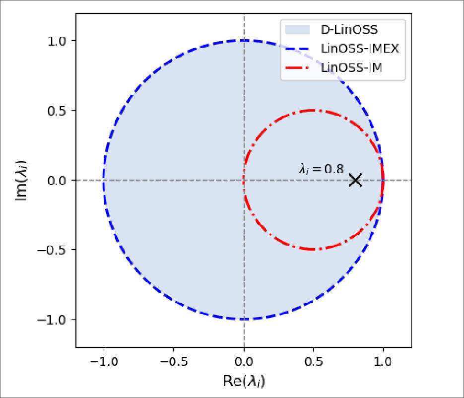
Solution: Dampened oscillator in continuous time system, with a second diagonal parameter \(G \succeq 0\):
- \(A_n\) sets frequency, \(G_n\) sets decay.
- LinOSS is the \(G = 0\) case.
Discretizing with IMEX, and writing \(S_n = 1 + \Delta_n G_n\):
- The modulus depends on \(G_n\) only, phase on \(A_n\) only.
- Damping and frequency are decoupled, and the reachable set is the full unit disk.
- Stability is enforced via constraint:
- \(\Delta = \sigma(\bar\Delta) \in (0,1)\)
- \(G = \mathrm{ReLU}(\bar G)\)
- \((G_n - \Delta_n A_n)^2 \le 4A_n\) .
Initialization
\((A_n, G_n) \mapsto \lambda_n\) is a bijection onto the punctured unit disk, so an eigenvalue distribution can be specified and solved back for the parameters:
Best-performing scheme: radially uniform \(\lvert\lambda_n\rvert \in [0.9, 1.0]\), uniform phase, then invert. This is the LRU annulus init reached by a different route.
Non-normal Transition
The LinOSS transition is modeled as a first-order recurrence via a non-normal block-diagonal matrix. This introduces possibility for transient growth of the state, even when eigenvalues are smaller than 1. Stability is guaranteed in the LTI case, but making components like \(G\), \(A\), \(\Delta_{n}\) time-varying makes the system unstable, even if eigenvalues are on the unit-disk.
Selective S4D-Real: Mamba
Mamba also uses Zero-Order Hold to discretize system, but step is input-selective.
- Since \(a_{n}\) is strictly negative, \(\Delta_{t}\) strictly positive => \(\bar A_{t,n} \in (0,1)\)
- System is stable decay.
- \(\Delta_{t}\rightarrow 0\) holds state, large \(\Delta_{t}\) resets state.
- \(\bar B_{t,n} \approx \Delta_t B_{t,n}\) is implementation only, not mentioned in paper.
- Since \(\Delta_{t}\) depends on \(x_{t}\), system is not LTI, requires associative scan.
Initialization: \(\nu_n^{\log} = \log n\) (so \(\nu_{n}\) is same as in S4D-Real)
Selective S4D-Lin: Oscillatory Mamba
Making LinOSS selective is difficult due to the non-normality of the transition, which makes it possible for transient growth to occur. However, Mamba formulation also works for complex-valued \(a_{n}\).
- Modulus is unchanged to Mamba, eigenvalues are the same.
- System is also stable.
- Same time-step gating.
- Phase \(\omega_{n}\) needs no constraint, doesn't affect eigenvalue magnitude.
- Complex input force \(B\in\mathbb{C}^{1, N}\) and readout \(C\in \mathbb{C}^{N,1}\).
Selective Tuning
Problem: Phase is coupled to mode, can't tune mode selectively to input. For example, the model can't tune to changing pitch while keeping magnitude. Introducing a second \(\Delta_{\theta}\) term so that \(\exp(-\Delta_t \nu_n) \cdot \exp(i\,\Delta_{\theta} \omega_n)\) looses continuous-time formulation => SSM can't adapt to differing STFT framerates.
Solution: Add input-dependent phase-offset so that model can selectively adapt to input.
The offset is also multiplied by time-step, so changing the framerate scales everything consistently. Still stable since only phase-angle is touched, modulus stays unchanged.